
Drawing Spirograph curves in Python

I was looking back over an old blog post and noticed some code in the comments that I had overlooked. Tom Pollard gives the following code for drawing Spirograph-like curves.
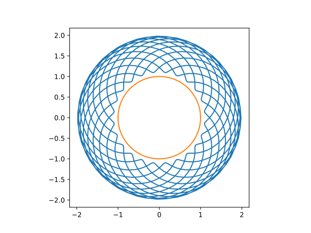
import matplotlib.pyplot as plt
from numpy import pi, exp, real, imag, linspace

def spiro(t, r1, r2, r3):
    """
    Create Spirograph curves made by one circle of radius r2 rolling 
    around the inside (or outside) of another of radius r1.  The pen
    is a distance r3 from the center of the first circle.
    """
    return r3*exp(1j*t*(r1+r2)/r2) + (r1+r2)*exp(1j*t)

def circle(t, r):
    return r * exp(1j*t)

r1 = 1.0
r2 = 52.0/96.0
r3 = 42.0/96.0

ncycle = 13 # LCM(r1,r2)/r2

t = linspace(0, ncycle*2*pi, 1000)
plt.plot(real(spiro(t, r1, r2, r3)), imag(spiro(t, r1, r2, r3)))
plt.plot(real(circle(t, r1)), imag(circle(t, r1)))
 
fig = plt.gcf()
fig.gca().set_aspect('equal')
plt.show()

Tom points out that with the r parameters above, this produces the default curve on Nathan Friend’s Inspirograph app.


from John D. Cook https://ift.tt/2Nb6HQF
via IFTTT

Comments

Popular posts from this blog

Controlling legend appearance in ggplot2 with override.aes

[This article was first published on Very statisticious on Very statisticious , and kindly contributed to R-bloggers ]. (You can report issue about the content on this page here ) Want to share your content on R-bloggers? click here if you have a blog, or here if you don't. In ggplot2 , aesthetics and their scale_*() functions change both the plot appearance and the plot legend appearance simultaneously. The override.aes argument in guide_legend() allows the user to change only the legend appearance without affecting the rest of the plot. This is useful for making the legend more readable or for creating certain types of combined legends. In this post I’ll first introduce override.aes with a basic example and then go through three additional plotting scenarios to how other instances where override.aes comes in handy. Table of Contents R packages Introducing override.aes Adding a guides() layer Using the guide argument in scale_*() Changing multiple aesthetic par...

Zooming in on maps with sf and ggplot2

(This article was first published on r-bloggers – WZB Data Science Blog , and kindly contributed to R-bloggers) When working with geo-spatial data in R, I usually use the sf package for manipulating spatial data as Simple Features objects and ggplot2 with geom_sf for visualizing these data. One thing that comes up regularly is “zooming in” on a certain region of interest, i.e. displaying a certain map detail. There are several ways to do so. Three common options are: selecting only certain areas of interest from the spatial dataset (e.g. only certain countries / continent(s) / etc.) cropping the geometries in the spatial dataset using sf_crop() restricting the display window via coord_sf() I will show the advantages and disadvantages of these options and especially focus on how to zoom in on a certain point of interest at a specific “zoom level”. We will see how to calculate the coordinates of the display window or “bounding box” around this zoom point. Loading t...