Turkey vs. Germany: COVID-19

[This article was first published on DataGeeek, and kindly contributed to R-bloggers]. (You can report issue about the content on this page here)

Want to share your content on R-bloggers? click here if you have a blog, or here if you don't.

In Turkey, some parts of society always compare Turkey to Germany and think that we are better than Germany for a lot of issues. The same applies to COVID-19 crisis management; is that reflects to true?

We will use two variables for compared parameters; the number of daily new cases and daily new deaths.First, we will compare the mean of new cases of the two countries. The dataset we’re going to use is here.

#load and tidying the dataset
library(readxl)

deu <- read_excel("covid-data.xlsx",sheet = "deu")
deu$date <- as.Date(deu$date)
tur <- read_excel("covid-data.xlsx",sheet = "tur")
tur$date <- as.Date(tur$date)

#building the function comparing means on grid table
grid_comparing <- function(column="new_cases"){

  table <-data.frame(
  deu=c(mean=mean(deu[[column]]),sd=sd(deu[[column]]),n=nrow(deu)),
  tur=c(mean=mean(tur[[column]]),sd=sd(tur[[column]]),n=nrow(tur))
) %>% round(2)

grid.table(table)
}

grid_comparing()

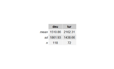
Above table shows that the mean of new cases in Turkey is greater than Germany. To check it, we will inference concerning the difference between two means.

In order to make statistical inference for the $\mu_1-\mu_2$ , the $\bar X_1-\bar X_2$ sample distribution must be approximately normal distribution. If it is assumed that the related populations will not be normal, $\bar X_1-\bar X_2$ sample distribution is approximately normal only in the volume of relevant samples greater than 30 separately according to the central limit theorem. In this case, the distribution is assumed approximately normal.

If the variances of two populations $\sigma_1^2$ and $\sigma_2^2$ are known, z-distribution would be used for statistical inference. A more common situation, if the variances of population are unknown, we will instead use samples variances $s_1^2$ , $s_2^2$ and $t_{sd}$ distribution.

When $\sigma_1^2$ and $\sigma_2^2$ are unknown, two situation are examined.

$\sigma_1^2=$ $\sigma_2^2$ : the assumption they are equal.
$\sigma_1^2\neq$ $\sigma_2^2$ : the assumption they are not equal.

There is a formal test to check whether population variances are equal or not which is a hypothesis test for the ratio of two population variances. A two-tailed hypothesis test is used for this as shown below.

$H_0: \sigma_1^2/\sigma_2^2=0$

$H_A: \sigma_1^2/\sigma_2^2\neq1$

The test statistic for $\sigma_1^2/\sigma_2^2$ :

$F_{(sd_1,sd_2)}=$ ${s_1^2}/{s_2^2}$

The sample volumes $n_1$ and $n_2$ , degrees of freedom of the samples $sd_1=n_1-1$ and $sd_2=n_2-1$ . F-distribution is used to describe the sample distribution of $S_1^2/S_2^2$

var.test(deu$new_cases,tur$new_cases)

#       F test to compare two variances

#data:  deu$new_cases and tur$new_cases
#F = 1.675, num df = 117, denom df = 71, p-value = 0.01933
#alternative hypothesis: true ratio of variances is not equal to 1
#95 percent confidence interval:
# 1.088810 2.521096
#sample estimates:
#ratio of variances 
#          1.674964

At the %5 significance level, because p-value(0.01933) is less than 0.05, the null hypothesis( $H_0$ ) is rejected and we assume that variances of the populations are not equal.

Because the variances are not equal we use Welch’s t-test to calculate test statistic:

$t_{sd}=$ $\frac{(\bar x_1-\bar x_2)} {\sqrt{(\frac{s_1^2} {n_1}+\frac{s_2^2} {n_2})}}$

The degree of freedom:

$sd=\frac{(s_1^2/n_1 + s_2^2/n_2)^2} {(s_1^2/n_1)^2/(n_1-1)+(s_2^2/n_2)^2/(n_2-1)}$

Let’s see whether the mean of new cases per day of Turkey( $\mu_1$ ) greater than Germany( $\mu_2$ ); to do that we will build the hypothesis test as shown below:

$H_0: \mu_1-\mu_2 \leq 0$

$H_A: \mu_1-\mu_2 > 0$

#default var.equal value is set to FALSE that indicates that the test is Welch's t-test
t.test(tur$new_cases,deu$new_cases,alternative = "g")

#       Welch Two Sample t-test

#data:  tur$new_cases and deu$new_cases
#t = 2.7021, df = 177.67, p-value = 0.00378
#alternative hypothesis: true difference in means is greater than 0
#95 percent confidence interval:
# 252.8078      Inf
#sample estimates:
#mean of x mean of y 
# 2162.306  1510.856

As shown above , at the %5 significance because the p-value(0.00378) is les than 0.05 the alternative hypothesis is accepted, which means in terms of controlling the spread of the disease, Turkey seems to be less successful than in Germany.

Another common thought in Turkish people that the health system in the country is much better than many European countries including Germany; let’s check that with daily death toll variable (new_deaths).

grid_comparing("new_deaths")

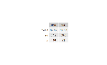
It seems Turkey has much less mean of daily deaths than Germany. Let’s check it.

var.test(deu$new_deaths,tur$new_deaths)

#       F test to compare two variances

#data:  deu$new_deaths and tur$new_deaths
#F = 4.9262, num df = 117, denom df = 71, p-value = 1.586e-11
#alternative hypothesis: true ratio of variances is not equal to 1
#95 percent confidence interval:
# 3.202277 7.414748
#sample estimates:
#ratio of variances 
#          4.926203

As described before, we will use Welch’s t-test because the variances are not equal as shown above(p-value = 1.586e-11 < 0.05).

t.test(deu$new_deaths,tur$new_deaths,alternative = "g")

#       Welch Two Sample t-test

#data:  deu$new_deaths and tur$new_deaths
#t = 1.0765, df = 175.74, p-value = 0.1416
#alternative hypothesis: true difference in means is greater than 0
#95 percent confidence interval:
# -5.390404       Inf
#sample estimates:
#mean of x mean of y 
# 69.88983  59.83333

At %5 significance level, alternative hypothesis is rejected(p-value = 0.1416 >0.05). This indicates that the mean of daily deaths of Germany is not worst than Turkey’s.

June 1 is set as the day of normalization by the Turkish government therefore many restrictions will be removed after that day. In order to check the decision, first, we will determine fit models for forecasting. To find the fit model we will build a function that compares trend regression models in a plot.

models_plot <- function(df=tur,column="new_cases"){
  
  df<- df[!df[[column]]==0,]#remove all 0 rows to calculate the models properly
  
  #exponential trend model data frame
  exp_model <- lm(log(df[[column]])~index,data = df) 
  exp_model_df <- data.frame(index=df$index,column=exp(fitted(exp_model)))
  names(exp_model_df)[2] <- column
  
  #comparing the trend plots
  ggplot(df,mapping=aes(x=index,y=.data[[column]])) + geom_point() +
    stat_smooth(method = 'lm', aes(colour = 'linear'), se = FALSE) +
    stat_smooth(method = 'lm', formula = y ~ poly(x,2), aes(colour = 'quadratic'), se= FALSE) +
    stat_smooth(method = 'lm', formula = y ~ poly(x,3), aes(colour = 'cubic'), se = FALSE)+
    stat_smooth(data=exp_model_df,method = 'loess',mapping=aes(x=index,y=.data[[column]],colour = 'exponential'), se = FALSE)+
    labs(color="Models",y=str_replace(column,"_"," "))+
    theme_bw()
 }

models_plot()

As we can see from the plot above, the cubic and quadratic regression models seem to fit the data more. To be able to more precise we will create a function that compares adjusted $R^2$ .

#comparing model accuracy
trendModels_accuracy <- function(df=tur,column="new_cases"){
  
  df<- df[!df[[column]]==0,]#remove all 0 rows to calculate the models properly
  
  model_quadratic <- lm(data = df,df[[column]]~poly(index,2))
  model_cubic <- lm(data = df,df[[column]]~poly(index,3))
  
  #adjusted coefficients of determination
  adj_r_squared_quadratic <- summary(model_quadratic) %>% 
    .$adj.r.squared
  
  adj_r_squared_cubic <- summary(model_cubic) %>% 
    .$adj.r.squared
  
  c(quadratic=round(adj_r_squared_quadratic,2),cubic=round(adj_r_squared_cubic,2))
  
}

trendModels_accuracy()
#quadratic     cubic 
#     0.73      0.77

The cubic trend regression model is much better than the quadratic trend model for Turkeys spread of disease as shown above.

Now, let’s find should the normalization day(June 1) is true. In the following code chunk, we will try some index numbers to find zero new cases.

#forecasting zero point for new cases in Turkey
model_cubic <- lm(formula = new_cases ~ poly(index, 3), data = tur)
predict(model_cubic,newdata=data.frame(index=c(77,78,79,80)))

#        1         2         3         4 
#183.92149 111.23894  42.50292 -22.04057

As shown above, index 80 goes to negative, so it can be considered as the day of normalization. If we look at the dataset, we can see that day is June 1. So the government seems to be right about the normalization calendar.

You can do the same predictions for Germany using the functions we created before.

To leave a comment for the author, please follow the link and comment on their blog: DataGeeek.

R-bloggers.com offers daily e-mail updates about R news and tutorials about learning R and many other topics. Click here if you're looking to post or find an R/data-science job.

Want to share your content on R-bloggers? click here if you have a blog, or here if you don't.

from R-bloggers https://ift.tt/2BeM0Pa
via IFTTT

The con behind every wedding

With her marriage on the rocks, one writer struggles to reconcile her cynicism about happily-ever-after as her own children rush to tie the knot A lavish wedding, a couple in love; romance was in the air, as it should be when two people are getting married. But on the top table, the mothers of the happy pair were bonding over their imminent plans for … divorce. That story was told to me by the mother of the bride. The wedding in question was two summers ago: she is now divorced, and the bridegroom’s parents are separated. “We couldn’t but be aware of the crushing irony of the situation,” said my friend. “There we were, celebrating our children’s marriage, while plotting our own escapes from relationships that had long ago gone sour, and had probably been held together by our children. Now they were off to start their lives together, we could be off, too – on our own, or in search of new partners.” Continue reading... The Guardian http://ift.tt/2xZTguV October 07, 2017 at 09:00AM

DataScience4you2me

Search This Blog

Turkey vs. Germany: COVID-19

Labels

Comments

Post a Comment

Popular posts from this blog

Former San Diego mayor joins race for California governor

Explaining models with Triplot, part 1

The con behind every wedding