Superfactorial

The factorial of a positive integer n is the product of the numbers from 1 up to and including n:

n! = 1 × 2 × 3 × … × n.

The superfactorial of n is the product of the factorials of the numbers from 1 up to and including n:

S(n) = 1! × 2! × 3! × … × n!.

For example,

S(5) = 1! 2! 3! 4! 5! = 1 × 2 × 6 × 24 × 120 = 34560.

Here are three examples of where superfactorial pops up.

Vandermonde determinant

If V is the n by n matrix whose ij entry is i^j-1 then its determinant is S(n-1). For instance,

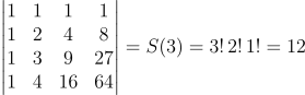
$\begin{vmatrix} 1 & 1 & 1 & 1 \\ 1 & 2 & 4 & 8 \\ 1 & 3 & 9 & 27 \\ 1 & 4 & 16& 64 \end{vmatrix} = S(3) = 3!\, 2!\, 1! = 12$

V is an example of a Vandermonde matrix.

Permutation tensor

One way to define the permutation symbol uses superfactorial:

$\epsilon_{i_1 i_2 \cdots i_n} = \frac{1}{S(n-1)} \prod_{1 \leq i < j \leq n} (i_j - i_k)$

Barnes G-function

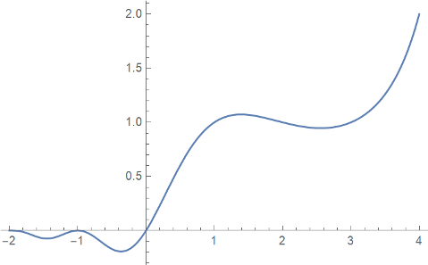
The Barnes G-function extends superfactorial to the complex plane analogously to how the gamma function extends factorial. For positive integers n,

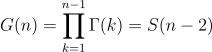
$G(n) = \prod_{k=1}^{n-1}\Gamma(k) = S(n-2)$

Here’s plot of G(x)

produced by

    Plot[BarnesG[x], {x, -2, 4}]

in Mathematica.

More posts related to factorial

The post Superfactorial first appeared on John D. Cook.

from John D. Cook https://ift.tt/3ixo5LM
via IFTTT

Comments

Former San Diego mayor joins race for California governor

Former San Diego Mayor Kevin Faulconer is running for California governorABC News: Top Stories https://ift.tt/3oNBFgt February 02, 2021 at 08:39AM

Controlling legend appearance in ggplot2 with override.aes

[This article was first published on Very statisticious on Very statisticious , and kindly contributed to R-bloggers ]. (You can report issue about the content on this page here ) Want to share your content on R-bloggers? click here if you have a blog, or here if you don't. In ggplot2 , aesthetics and their scale_*() functions change both the plot appearance and the plot legend appearance simultaneously. The override.aes argument in guide_legend() allows the user to change only the legend appearance without affecting the rest of the plot. This is useful for making the legend more readable or for creating certain types of combined legends. In this post I’ll first introduce override.aes with a basic example and then go through three additional plotting scenarios to how other instances where override.aes comes in handy. Table of Contents R packages Introducing override.aes Adding a guides() layer Using the guide argument in scale_*() Changing multiple aesthetic par...

Using RStudio and LaTeX

(This article was first published on r – Experimental Behaviour , and kindly contributed to R-bloggers) This post will explain how to integrate RStudio and LaTeX, especially the inclusion of well-formatted tables and nice-looking graphs and figures produced in RStudio and imported to LaTeX. To follow along you will need RStudio, MS Excel and LaTeX. Using tikzdevice to insert R Graphs into LaTeX I am a very visual thinker. If I want to understand a concept I usually and subconsciously try to visualise it. Therefore, more my PhD I tried to transport a lot of empirical insights by means of visualization . These range from histograms, or violin plots to show distributions, over bargraphs including error bars to compare means, to interaction- or conditional effects of regression models. For quite a while it was very tedious to include such graphs in LaTeX documents. I tried several ways, like saving them as pdf and then including them in LaTeX as pdf, or any other file ...

DataScience4you2me

Search This Blog