This post will look at simple numerical approaches to solving the preditor-prey (Lotka-Volterra) equations. It turns out that the simplest approach does poorly, but a slight variation does much better.
Following [1] we will use the equations
u‘ = u (v – 2)
v‘ = v (1 – u)
Here u represents the predator population over time and v represents the prey population. When the prey v increase, the predators u increase, leading to a decrease in prey, which leads to a decrease in predators, etc. The exact solutions are periodic.
Euler’s method replaces the derivatives with finite difference approximations to compute the solution in increments of time of size h. The explicit Euler method applied to our example gives
u(t + h) = u(t) + h u(t) (v(t) – 2)
v(t + h) = v(t) + h v(t) (1 – u(t)).
The implicit Euler method gives
u(t + h) = u(t) + h u(t + h) (v(t + h) – 2)
v(t + h) = v(t) + h v(t + h) (1 – u(t + h)).
This method is implicit because the unknowns, the value of the solution at the next time step, appear on both sides of the equation. This means we’d either need to do some hand calculations first, if possible, to solve for the solutions at time t + h, or use a root-finding method at each time step to solve for the solutions.
Implicit methods are more difficult to implement, but they can have better numerical properties. See this post on stiff equations for an example where implicit Euler is much more stable than explicit Euler. I won’t plot the implicit Euler solutions here, but the implicit Euler method doesn’t do much better than the explicit Euler method in this example.
It turns out that a better approach than either explicit Euler or implicit Euler in our example is a compromise between the two: use explicit Euler to advance one component and use implicit Euler on the other. This is known as symplectic Euler for reasons I won’t get into here but would like to discuss in a future post.
If we use explicit Euler on the predator equation but implicit Euler on the prey equation we have
u(t + h) = u(t) + h u(t) (v(t + h) – 2)
v(t + h) = v(t) + h v(t + h) (1 – u(t)).
Conversely, if we use implicit Euler on the predator equation but explicit Euler on the prey equation we have
u(t + h) = u(t) + h u(t + h) (v(t) – 2)
v(t + h) = v(t) + h v(t) (1 – u(t + h)).
Let’s see how explicit Euler compares to either of the symplectic Euler methods.
First some initial setup.
    import numpy as np

    h  = 0.08  # Step size
    u0 = 6     # Initial condition
    v0 = 2     # Initial condition
    N  = 100   # Numer of time steps

    u = np.empty(N)
    v = np.empty(N)
    u[0] = u0
    v[0] = v0
Now the explicit Euler solution can be computed as follows.
    for n in range(N-1):
        u[n+1] = u[n] + h*u[n]*(v[n] - 2)
        v[n+1] = v[n] + h*v[n]*(1 - u[n])
The two symplectic Euler solutions are
    for n in range(N-1):
        v[n+1] = v[n]/(1 + h*(u[n] - 1))
        u[n+1] = u[n] + h*u[n]*(v[n+1] - 2)
and
    for n in range(N-1):
        u[n+1] = u[n] / (1 - h*(v[n] - 2))
        v[n+1] = v[n] + h*v[n]*(1 - u[n+1])
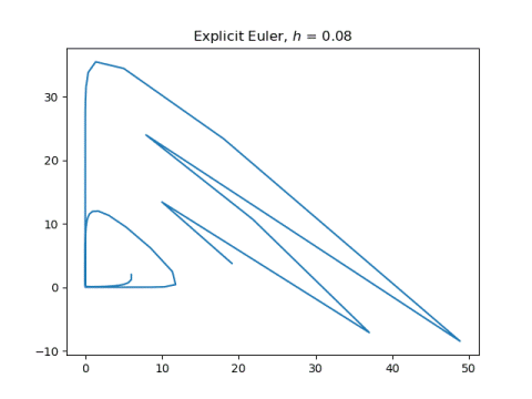
Now let’s see what our solutions look like. First explicit Euler applied to both components:
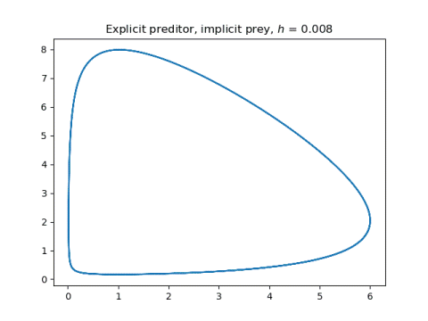
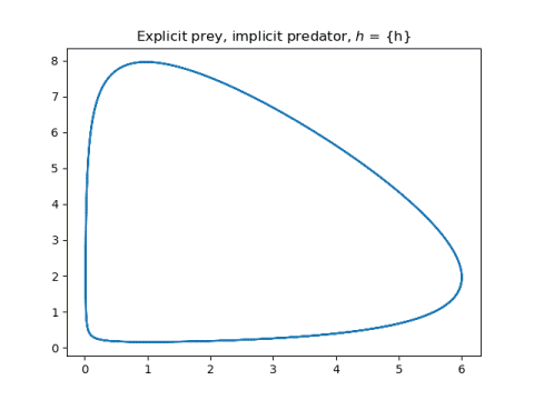
And now the two symplectic methods, applying explicit Euler to one component and implicit Euler to the other.
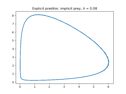
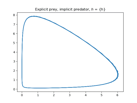
Next, let’s make the step size 10x smaller and the number of steps 10x larger.
Now the explicit Euler method does much better, though the solutions are still not quite periodic.
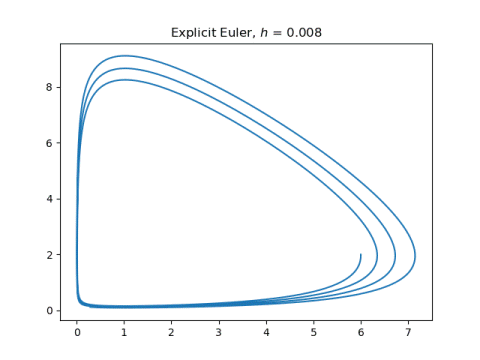
The symplectic method solutions hardly change. They just become a little smoother.
More differential equations posts
[1] Ernst Hairer, Christian Lubich, Gerhard Wanner. Geometric Numerical Integration: Structure-Preserving Algorithms for Ordinary Differential Equations.
The post Symplectic Euler first appeared on John D. Cook.
from John D. Cook https://ift.tt/2Fwz0GZ
via IFTTT
Comments
Post a Comment